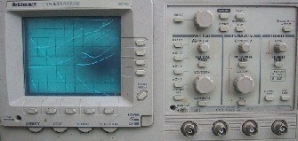
The photograph on the left shows a 4-Channel 200MHz oscilloscope. While no two models of oscilloscope are the same, they are very similar. The number of channels available and the bandwidth are the primary differences as discussed previously. Some units have various extra features, such as on-screen displays and measurement tools.
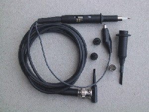
To use the oscilloscope we will need a probe. A typical probe is shown on the right. They are supplied with a selection of adaptors (the round objects in the photograph), a hook device so we can physically attach the probe to the measurement point, and a trimming tools so we can match the probe to the oscilloscope.
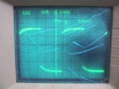 As
supplied, the probe will probably be a poor match for our oscilloscope. The
trace shown on the right should be a square wave, but notice that the leading
edges of each transition are rounded. We must match the probe to the
oscilloscope, by making the capacitance of both equal. We achieve this by
adjusting a variable capacitor inside the body of the probe. In the photograph
of the probe above, you may notice a small hole in the body with a screw-slot
adjustment behind the hole. This is why a trimming tool is supplied. Do not use
a metal tool, it's presence may affect the electronics in the probe and lead to
incorrect adjustment. We connect the probe to the test terminal on the
oscilloscope which supplies a 1KHz square wave at about 5V.
As
supplied, the probe will probably be a poor match for our oscilloscope. The
trace shown on the right should be a square wave, but notice that the leading
edges of each transition are rounded. We must match the probe to the
oscilloscope, by making the capacitance of both equal. We achieve this by
adjusting a variable capacitor inside the body of the probe. In the photograph
of the probe above, you may notice a small hole in the body with a screw-slot
adjustment behind the hole. This is why a trimming tool is supplied. Do not use
a metal tool, it's presence may affect the electronics in the probe and lead to
incorrect adjustment. We connect the probe to the test terminal on the
oscilloscope which supplies a 1KHz square wave at about 5V.
 This
gives us a trace such as that shown in the above photograph. Now we must adjust
the probe until the tops of the square wave are as flat as possible, to give a
trace such as shown in the photo below. The probe is now a good match to the
oscilloscope and ready for us to use.
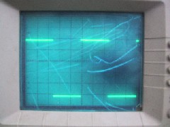
This
gives us a trace such as that shown in the above photograph. Now we must adjust
the probe until the tops of the square wave are as flat as possible, to give a
trace such as shown in the photo below. The probe is now a good match to the
oscilloscope and ready for us to use.
Now let's look at some measurements. As said on the previous page, the
oscilloscope's main job is not that of precise measurement. Rather it is used
for peaking or nulling signals (adjusting to maximum or minimum) or in
fault-finding, to detect the presence or absence of a signal. Nevertheless it is
often useful to be able to approximate the characteristics of a waveform. For
example, if we were fault-finding a frequency doubler circuit, it would be
useful to be able to visually verify that the circuits output was double, not
quadruple, its input frequency.
The
screen of an oscilloscope is divided into marked 1cm squares. In the photograph
on the right, we can see from the on-screen display, that the unit is set to
1V/cm on the Y-axis, and 200μs/cm (200 microseconds per centimetre) on the
X-axis.
By counting the number of squares between the maximum and minimum value, 5, and multiplying by the Y-axis setting (1V/cm) we can say that the waveform is approximately 5V peak to peak.
By counting the number of squares occupied by one cycle of the waveform, 5, and multiplying by the X-axis setting (200μs/cm) we can say that the waveform period is approximately 1000μs or 1ms, and thus that the frequency is approximately 1kHz.
Note that we cannot be any more precise than this.